Introduction

In two earlier posts, Adaptive PI Control with Python and MIMO Adaptive Control with Python, some simple adaptive control examples were presented along with some simulations demonstrating their performance. This post shares a third adaptive control example. Here, a controller from a 1994 paper by S.P. Karason and A.M. Annaswamy, Adaptive Control in the Presence of Input Constraints is presented and the simulation results are reproduced, again using the Python Control Systems Library.

Problem Statement

Consider the following standard scalar plant, reference model, and control law, but note the difference between the control law which produces the desired control $u_{c}$ and the control input $u$ to the plant. As before $a_{m}<0$, and the sign of $b_{p}$ is known.

\begin{align} &\mbox{Plant:} &\hspace{0.5in} \dot x_{p}&=a_{p}x_{p}+b_{p}u\label{eqn.plant} \\ &\mbox{Reference model:} &\hspace{0.5in} \dot x_{m}&=a_{m}x_{m}+b_{m}r\label{eqn.refmodel} \\ &\mbox{Control law:} &\hspace{0.5in} u_{c}&=\theta{} x_{p}+kr\label{eqn.adaptive.saturation.uc} \end{align}

Depending on the values of the adaptive parameters $\theta$ and $k$, the state $x_{p}$ and the reference input $r$, the desired control $u_{c}$ might be larger than what the actuator is actually capable of as given by $u$. This is known as actuator saturation, which all real actuators will have. This limit is a known constraint, for example how much torque a motor can apply, or how much a control surface on an aircraft can deflect. This limit can be modeled using $u_{\text{max}}>0$ such that $|u|\leq u_{\text{max}}$, after which the actuator experiences saturation. This saturation model can be expressed as follows.

\begin{align} \label{eqn.adaptive.saturation.usat} &\mbox{Control input:} &\hspace{0.5in} u&= \begin{cases} u_{c} &\mbox{if } |u_{c}|\leq{} u_{\text{max}} \\ u_{\text{max}}\text{sgn}(u_{c}) & \mbox{if } |u_{c}|>u_{\text{max}} \end{cases} \end{align}

Before considering a control solution which accommodates the actuator saturation in \eqref{eqn.adaptive.saturation.usat}, the case where the actuator has no saturation limits will be quickly reviewed first. That is set $u=u_{c}$ and design a controller, resulting in the standard adaptive system outlined below. The tracking and parameter error are given by

\begin{equation}\label{eqn.adaptive.saturation.e} e=x_{p}-x_{m} \end{equation}

and parameter error as

\begin{equation}\label{eqn.adaptive.saturation.param_errors} \tilde{\theta~}=\theta-\theta^{*}\hspace{0.5in}\tilde{k~}=k-{k}^{ *} \end{equation}

with matching conditions

\begin{equation}\label{eqn.adaptive.saturation.matching} a_{m}=a_{p}+b_{p}\theta^{*} \hspace{0.5in} b_{m}=b_{p}k^{*} \end{equation}

and error dynamics

\begin{equation*} \dot{e}=a_{m}e+b_{p}\tilde{\theta}x_{p}+b_{p}\tilde{k}r \end{equation*}

Using the following standard update laws in \eqref{standard.update.laws}, stability can easily be proved.

\begin{equation} \label{standard.update.laws} \mbox{Update laws:}\hspace{0.5in}
\begin{array}{l} \dot{\tilde{k~}}=-\text{sgn}(b_{p})er \\ \dot{\tilde{\theta~}}=-\text{sgn}(b_{p})ex_{p} \end{array} \end{equation}

But when these standard adaptive laws are used in the presence of the actuator constraints in \eqref{eqn.adaptive.saturation.usat} the system is no longer globally stable and behaves undesirably. An adaptive controller that accommodates the actuator limitations in \eqref{eqn.adaptive.saturation.usat} is desired.

The Adaptive Controller

In what follows, modifications to the adaptive system presented above will be proposed so as to provide stability in the presence of the actuator saturation model in \eqref{eqn.adaptive.saturation.usat}. The control input can be expressed in two parts: the total desired control as computed by the control law, and a component which subtracts off the portion of this control signal which the actuator is unable to produce. These components are $u_{c}$ and $\Delta u$, respectively, where $\Delta u$ is the control deficit. Because the desired control and control input are known quantities, so is the control deficit. The control input can be expressed

\begin{align}\label{eqn.adaptive.saturation.u} u=u_{c}+\Delta{}u \end{align}

Substituting \eqref{eqn.adaptive.saturation.u} into the plant equation \eqref{eqn.plant} with control law \eqref{eqn.adaptive.saturation.uc} the plant dynamics can be written

\begin{equation}\label{eqnxpdot} \dot x_{p}=(a_{p}+b_{p}\theta)x_{p}+b_{p}kr+b_{p}\Delta u \end{equation}

Differentiating the tracking error \eqref{eqn.adaptive.saturation.e} and using \eqref{eqnxpdot} and \eqref{eqn.refmodel} along with the matching conditions \eqref{eqn.adaptive.saturation.matching} and parameter errors \eqref{eqn.adaptive.saturation.param_errors} gives the following error dynamics

\begin{align}\label{eqn.adaptive.saturation.edot} \dot{e}=a_{m}e+b_{p}\tilde{\theta~}x_{p}+b_{p}\tilde{k~}r+b_{p}\Delta{}u \end{align}

The control deficit $\Delta u$, can be looked at like a disturbance to the system that the adaptive scheme must deal with. The adaptive system should only try to reduce the portion of the error which it actually has the actuator authority to do so. This controllable error $e_{u}$ is given by

\begin{equation}\label{eqn.controllable_error} e_{u}=e-e_{\Delta} \end{equation}

The controllable error is obtained by subtracting the deficit error $e_{\Delta}$ from the tracking error. The deficit error, the portion of the error beyond the limits of the actuator to control, is due to $\Delta u$ and is determined from the following differential equation, where the input $\beta_{\Delta}$ is unknown.

\begin{equation}\label{eqn.adaptive.saturation.edeltadot} \dot e_{\Delta}=a_{m}e_{\Delta}+\beta_{\Delta}\Delta{}u \end{equation}

When the control input is saturating, the controller cannot achieve any higher level of performance. That is, the controller should not seek to minimize an error signal beyond the limitations of the actuator authority. Instead the error $e_{u}$ is defined, which takes the tracking error and subtracts off the portion due to the “disturbance” $\Delta u$ which the controller, limited by the actuator, can do nothing about. It is this is controllable error that should drive adaptation. If the controller is saturating the actuator, there is no sense using an error signal which the controller cannot reduce to drive adaptation – this will only lead to wind-up. The last adaptive parameter error term is defined as

\begin{equation}\label{eqn.adaptive.saturation.beta_tilde} \tilde{\beta~}=b_{p}-\beta_{\Delta} \end{equation}

The dynamics describing the controllable error are given by differentiating \eqref{eqn.controllable_error} and using \eqref{eqn.adaptive.saturation.edot} and \eqref{eqn.adaptive.saturation.edeltadot}, finally giving the following controllable error dynamics

\begin{equation}\label{eqn.adaptive.saturation.eudot} \dot e_{u}=a_{m}e_{u}+b_{p}\tilde{\theta~}x_{p}+b_{p}\tilde{k~}r+\tilde{\beta~}\Delta{}u \end{equation}

Again, this is the error which the controller should try to minimize. Propose the following candidate Lyapunov function

\begin{equation*} V(e_{u},\tilde{\theta~},\tilde{k~},\tilde{\beta~})= \frac{1}{2}e_{u}{}^{2}+ \frac{1}{2}|b_{p}|\gamma_{1}^{-1}\tilde{\theta~}^{2}+ \frac{1}{2}|b_{p}|\gamma_{2}^{-1}\tilde{k~}^{2}+ \frac{1}{2}\gamma_{3}^{-1}\tilde{\beta~}^{2} \end{equation*}

Differentiating and using the following update laws

\begin{align*} \dot{\tilde{\theta~}}&=-\gamma_{1}\text{sgn}(b_{p})e_{u}x_{p} \\ \dot{\tilde{k~}}&=-\gamma_{2}\text{sgn}(b_{p})e_{u}r \\ \dot{\tilde{\beta~}}&=-\gamma_{3}e_{u}\Delta u \end{align*}

gives

\begin{equation*} \dot{V}=a_{m}e_{u}{}^{2}\leq0 \end{equation*}

From this it follows that $e_{u}$, $\tilde{\theta~}$, $\tilde{k~}$, and $\tilde{\beta~}$ are bounded $\forall t\geq t_{0}$. The rest of the stability proof is omitted, but the main point, one that should not be unexpected, is that stability is local. Even in the nonadaptive case a local stability result should be expected – global stability of an unstable plant cannot be guaranteed given limited actuator authority. Bounds are provided within which local stability is provided and the errors $e_{u}(t)$ and $e(t)$ tend to zero as $t\rightarrow\infty$.

Simulation Result

As usual, the code to create these simulations is available on Github: dpwiese/control-examples/saturation-protection. None of the code is presented or described here as the implementation is quite straightforward. Note that in the paper the values for the gains $\gamma_{1}$, $\gamma_{2}$, and $\gamma_{3}$ are not given, so the values used in the simulations were selected to as to produce similar results to those in the paper.

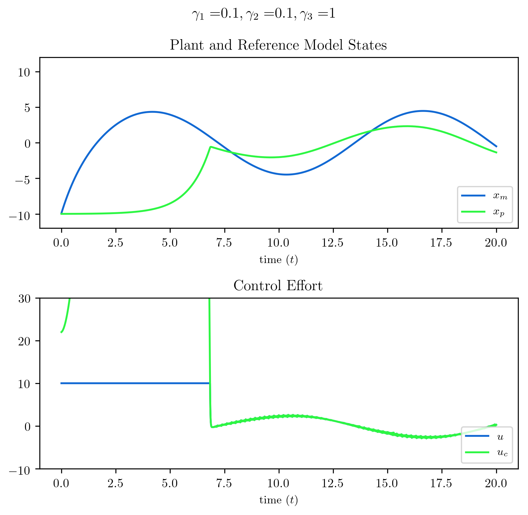
The reference input in both plots below is $r(t)=\text{sin}(0.5t)$ and control saturation $u_{\text{max}}=10$. The first plot shows the result of the method presented above. The controller, while saturating the actuator for the first six seconds or so, handles this saturation well – it does not increase the desired control too much beyond the actuator’s capabilities. As the tracking error is reduced and the desired control is within the actuator’s limits, the controller quickly and smoothly brings the tracking error near zero by about ten seconds in and maintains a good response for the duration of the simulation.

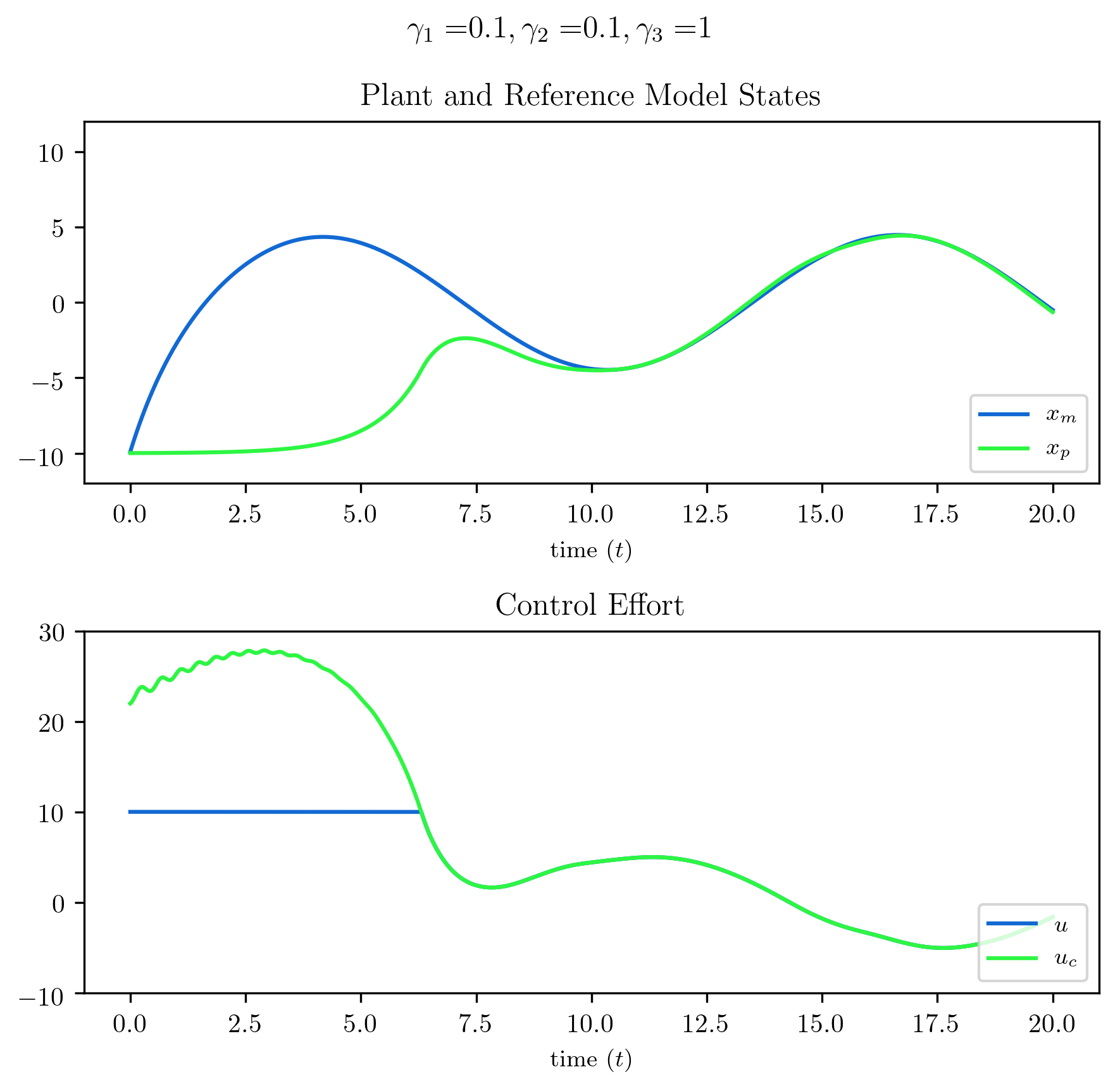
The second plot illustrates what happens if the method presented above is not used. Here it can be seen for the first six seconds or so, while the actuator is saturating, the desired control continues to increase, winding up as the tracking error remains nonzero until around seven seconds. As the tracking error decreases towards zero, the desired control abruptly decreases, and for the duration of the simulation never manages to really track the reference.