Introduction

In a previous post, Adaptive PI Control with Python, an example of an adaptive PI controller was presented and the Python Control Systems Library used to simulate the closed-loop response. This was a simple academic problem well suited to demonstrating the abilities of the library. Since then I’ve been re-implementing various other simulation examples as well. The current post presents a more complex example of a classical multi-input multi-output adaptive system. No attempt is made to explain the steps in the open-loop analysis or control synthesis, or prove stability - they are simply presented as-is. For more details on the design of such a controller see Reference ¹. This post is meant only as a quick walkthrough to share another example of the Python Control Systems Library in action.

Open-Loop System

Consider the following LTI plant

\begin{equation*} \begin{split} \dot{x}&=Ax+Bu \\ y_{p}&=Cx \end{split} \end{equation*}

where $x\in\mathbb{R}^{n}$, $y_{p}\in\mathbb{R}^{p}$, and $u\in\mathbb{R}^{m}$ and the system matrices are given by

\begin{equation}\label{eqn-adaptive-plantmatrices} A= \begin{bmatrix} -2 & -1 & 0 & 0 & 0 \\ 1 & 0 & 0 & 0 & 0 \\ 0 & 0 & -4 & -2 & 0 \\ 0 & 0 & 2 & 0 & 0 \\ 0 & 0 & 0 & 0 & 3 \end{bmatrix} \qquad B= \begin{bmatrix} 1 & 0 \\ 0 & 0 \\ 0 & 1 \\ 0 & 0 \\ 0 & 1 \end{bmatrix} \qquad C= \begin{bmatrix} 1 & 1 & 0 & 1 & 0 \\ 0 & 1 & 0 & 0 & 1 \end{bmatrix} \end{equation}

The system is fifth order with two inputs and two outputs; that is $n=5$, $m=2$, and $p=2$. The system transfer matrix $W_{p}(s)$ is defined as follows

\begin{equation*} W_{p}(s)\triangleq C(sI-A)^{-1}B\in\mathbb{R}_{p}^{p\times m}(s) \end{equation*}

and for the system with matrices in \eqref{eqn-adaptive-plantmatrices} gives

\begin{equation*} W_{p}(s)= \begin{bmatrix} \frac{1}{s+1}& \frac{2}{(s+2)^{2}} \\ \frac{1}{(s+1)^{2}} & \frac{1}{s-3} \end{bmatrix} \end{equation*}

Note that while the system above has been defined with values to better illustrate the process of the control design, it is considered unknown. The extent to which the values need not be known is described in the steps below. Alternatively, had the plant been defined parametrically, the same analysis and control design could have been performed for some large set of these parameters and the values substituted in when running the simulation.

Requirements

First, several requirements must be checked to determine whether the intended classical adaptive controller is applicable to the system in \eqref{eqn-adaptive-plantmatrices}. These requirements are:

1. Plant must be square, that is $m=p$.
2. The plant has no unstable transmission zeros.
   • This is to ensure pole-zero cancellations do not occur in the right half plane.
3. The Hermite form $H_{p}(s)$ of $W_{p}(s)$ is diagonal.
   • The only information needed to determine whether the Hermite form $H_{p}(s)$ of $W_{p}(s)$ is diagonal is the relative degree of each entry of $W_{p}(s)$.
4. The sign of the high frequency gain satisfies a sign definite condition.
5. An upper bound on the observability index is known.

In what follows we will verify that these requirements are satisfied, select a suitable reference model, define the control filters and finally assembled these various pieces resulting in the completed controller. These requirements are not particularly stringent, and do not require much information about the plant to verify. The resulting controller is not dependent on the particulars of the plant, so long as it satisfied the above requirements.

Evaluate System Transmission Zeros

This is accomplished by determining the system’s Smith-McMillan form, which useful in obtaining the poles and zeros (with their multiplicities) from a given transfer matrix. The Smith-McMillan form is found by dividing the system’s Smith Form by the minimum polynomial $d(s)$.

First calculate the minimum polynomial $d(s)$ of $W_{p}(s)$ as:

\begin{equation*} d(s)=(s+1)^{2}(s+2)^2(s-3) \end{equation*}

and express $W_{p}(s)$ as

\begin{equation*} W_{p}(s)=\frac{1}{d(s)}P(s) \end{equation*}

giving

\begin{equation*} P(s)= \begin{bmatrix} (s+1)(s+2)^{2}(s-3) & 2(s+1)^{2}(s-3) \\ (s+2)^{2}(s-3) & (s+1)^{2}(s+2)^{2} \end{bmatrix} \end{equation*}

Find the Smith form of $P(s)$ by finding the determinantal devisors as follows, with $D_{0}\triangleq1$. The $1\times1$ minors of $P(s)$ are:

\begin{equation*} (s+1)(s+2)^{2}(s-3) \qquad 2(s+1)^{2}(s-3) \qquad (s+2)^{2}(s-3) \qquad (s+1)^{2}(s+2)^{2} \end{equation*}

The greatest common devisor of these matrices is 1, so we set

\begin{equation*} D_{1}(s)=1 \end{equation*}

The $2\times2$ minor of $W_{p}(s)$ is:

\begin{equation*} (s+1)^{3}(s+2)^{4}(s-3)-2(s+1)^{2}(s+2)^{2}(s-3)^{2} = (s+1)^{2}(s+2)^{2}(s-3)[(s+1)(s+2)^{2}-2(s-3)] \end{equation*}

The greatest common devisor of this is itself, so we set

\begin{equation*} D_{2}(s)=(s+1)^{2}(s+2)^{2}(s-3)[(s+1)(s+2)^{2}-2(s-3)] \end{equation*}

Calculate $\epsilon_{i}^{\prime}$ as

\begin{equation*} \epsilon_{i}’(s)=\frac{D_{i}(s)}{D_{i-1}(s)} \end{equation*}

giving

\begin{equation*} \begin{split} \epsilon_{1}^{\prime}(s)&=1 \\ \epsilon_{2}^{\prime}(s)&=(s+1)^{2}(s+2)^{2}(s-3)[(s+1)(s+2)^{2}-2(s-3)] \end{split} \end{equation*}

So the Smith form of $P(s)$ is

\begin{equation*} S_{P}(s)= \begin{bmatrix} 1 & 0 \\ 0 & (s+1)^{2}(s+2)^{2}(s-3)[(s+1)(s+2)^{2}-2(s-3)] \end{bmatrix} \end{equation*}

To get the Smith-McMillan form of $W_{p}(s)$ divide the Smith form $S_{P}(s)$ by the minimum polynomial $d(s)$.

\begin{equation*} \begin{split} SM_{W_{p}}(s)&= \frac{1}{(s+1)^{2}(s+2)^2(s-3)} \begin{bmatrix} 1 & 0 \\ 0 & (s+1)^{2}(s+2)^{2}(s-3)[(s+1)(s+2)^{2}-2(s-3)] \end{bmatrix} \\ &= \begin{bmatrix} \frac{1}{(s+1)^{2}(s+2)^2(s-3)} & 0 \\ 0 & (s+1)(s+2)^{2}-2(s-3) \end{bmatrix} \end{split} \end{equation*}

Each of the diagonal entries of the Smith-McMillan form can be written as

\begin{equation*} \frac{\epsilon_{i}(s)}{\psi_{i}(s)} \end{equation*}

with

\begin{equation*} \begin{split} \epsilon_{1}&=1 \\ \epsilon_{2}&=(s+1)(s+2)^{2}-2(s-3) \end{split} \end{equation*}

and

\begin{equation*} \begin{split} \psi_{1}&=(s+1)^{2}(s+2)^2(s-3) \\ \psi_{2}&=1 \end{split} \end{equation*}

And so the characteristic polynomial $p(s)$ can be calculated as

\begin{equation*} \begin{split} p(s)&=\psi_{1}(s)\psi_{2}(s) \\ &=(s+1)^{2}(s+2)^2(s-3) \end{split} \end{equation*}

The zero polynomial is given by

\begin{equation*} \begin{split} z(s)&=\epsilon_{1}(s)\epsilon_{2}(s) \\ &=(s+1)(s+2)^{2}-2(s-3) \\ &=s^{3}+5s^{2}+6s+10 \end{split} \end{equation*}

We can see that this system is fifth order $n=5$, with a pole with multiplicity two at $s=-1$, a pole with multiplicity two at $s=-2$, and a pole at $s=3$. It also has three stable transmission zeros, as verified using the Routh–Hurwitz Stability Criterion. The exact location of the transmission zeros is not important.

Check Structure of Plant’s Hermite Form

Check the matrix $E$ to see if it is nonsingular. If so, the Hermite form $H_{p}(s)$ of $W_{p}(s)$ is diagonal, which will make control design easier, as described in Reference ¹, p. 396:

Dynamic decoupling of a MIMO plant, in which one output is affected by one and only one input, is obviously a desirable feature in multivariable control. If, by a suitable choice of a controller, a MIMO plant can be decoupled, then SISO control methods can be used for each loop to obtain the desired closed-loop response. It is clear that, given a transfer matrix $T(s)$, whether or not it can be decoupled is closely related to the Hermite normal form of $T(s)$. A diagonal Hermite form implies that the MIMO plant can be dynamically decoupled with a causal feedforward controller, or more realistically (to avoid unstable pole-zero cancellations), using an equivalent feedback controller. As seen in the following sections, in the adaptive control problem, only plants with diagonal Hermite normal forms can be realistically adaptively controlled in a stable fashion.

To do this, we first find the minimum relative degree $n_{i}$ of the elements in each row of $W_{p}(s)$.

\begin{equation*} \begin{split} n_{1}&=1 \\ n_{2}&=1 \end{split} \end{equation*}

Evaluate $E$

\begin{equation*} E_{i}=\lim_{s\rightarrow\infty}s^{r_{i}}G_{i}(s) \end{equation*}

where $G_{i}(s)$ corresponds to the $i^{\text{th}}$ row of $G(s)$. This gives

\begin{equation*} E_{1}=\lim_{s\rightarrow\infty}s \begin{bmatrix} \frac{1}{s+1} & \frac{2}{(s+2)^{2}} \end{bmatrix}= \begin{bmatrix} 1 & 0 \end{bmatrix} \end{equation*}

and

\begin{equation*} E_{2}=\lim_{s\rightarrow\infty}s \begin{bmatrix} \frac{1}{(s+1)^{2}} & \frac{1}{s-3} \end{bmatrix}= \begin{bmatrix} 0 & 1 \end{bmatrix} \end{equation*}

So

\begin{equation*} E= \begin{bmatrix} 1 & 0 \\ 0 & 1 \end{bmatrix} \end{equation*}

and since $E$ is nonsingular, the plant’s Hermite form $H_{p}(s)$ is diagonal.

Expressing the Plant’s Hermite Form

The plant’s Hermite form is given by

\begin{equation*} H_{p}(s)= \begin{bmatrix} \frac{1}{\pi^{n_{1}}(s)} & 0 & \cdots & 0 \\ 0 & \frac{1}{\pi^{n_{2}}(s)} & & \vdots \\ \vdots & & \ddots & 0 \\ 0 & \cdots & 0 & \frac{1}{\pi^{n_{m}}(s)} \end{bmatrix} \end{equation*}

where $\pi(s)$ is any monic polynomial of degree 1 and $n_{i}$ is the minimum relative degree of the elements of $W_{p}(s)$ in the $i^{\text{th}}$ row.

With $n_{1}=1$ and $n_{2}=1$ this gives

\begin{equation}\label{eqn-adaptive-hermiteform} H_{p}(s)= \begin{bmatrix} \frac{1}{(s+a)} & 0 \\ 0 & \frac{1}{(s+a)} \end{bmatrix} \end{equation}

Controller Synthesis

Find the High Frequency Gain

To find $K_{p}$, use $K_{p}=\lim_{s\rightarrow\infty}H_{p}^{-1}(s)W_{p}(s)$, which for diagonal Hermite forms is the same as $K_{p}=E[W_{p}(s)]$. So

\begin{equation*} K_{p}= \begin{bmatrix} 1 & 0 \\ 0 & 1 \end{bmatrix} \end{equation*}

From this it is clear that the high frequency gain satisfies the sign-definiteness condition. Note again that the particular values that arose from $E$ were not so important to satisfy this condition, and that it was the diagonality of $H_{p}(s)$ that gave $K_{p}$ this simple structure.

Select the Reference Model

Pick the reference model transfer matrix $W_{m}(s)$ as

\begin{equation*} W_{m}(s)=H_{p}(s)Q_{m}(s) \end{equation*}

where $Q_{m}(s)$ is an asymptotically stable unimodular matrix. For purposes of simplicity we can assume that $Q_{m}=\gamma I$, where $\gamma$ is picked so that the DC gain of the components of the diagonal Hermite form, and thus reference model, have unity DC gain. With $H_{p}(s)$ in \eqref{eqn-adaptive-hermiteform} and setting $\gamma=a$ this gives

\begin{equation}\label{eqn-adaptive-refmodel} W_{m}(s)= \begin{bmatrix} \frac{a}{(s+a)} & 0 \\ 0 & \frac{a}{(s+a)} \end{bmatrix} \end{equation}

Calculate an Upper Bound on the Observability Index

Calculate an upper bound $\nu$ on the observability index using the following from Reference ¹, p.406. It says an upper bound $\nu$ on the observability index can be obtained by knowing an upper bound $n_{ij}$ on the order of the $ij^{\text{th}}$ scalar entry in $W_{p}(s)$.

\begin{equation*} \nu=\left[\frac{1}{m}\sum_{i,j}n_{ij}\right] \end{equation*}

For this example, with $m=2$ and $n_{ij}$ determined by inspection $\nu$ is calculated as

\begin{equation*} \nu=\frac{1}{2}(1+2+2+1)=3 \end{equation*}

Design Controller Filters

Using the upper bound on the observability index $\nu$, we design $\nu-1$ control input filters, and $\nu$ output filters as follows, where $r_{q}(s)$ is a Hurwitz, monic polynomial of degree $\nu-1$.

\begin{align*} \mbox{Filtered control} \qquad & \omega_{i}(t)=\frac{s^{i-1}}{r_{q}(s)}u(t) \qquad i=1,\dots\nu-1 \\ \mbox{Filtered output} \qquad & \omega_{j}(t)=\frac{s^{j-1}}{r_{q}(s)}y_{p}(t) \qquad j=\nu,\dots2\nu-1 \\ \end{align*}

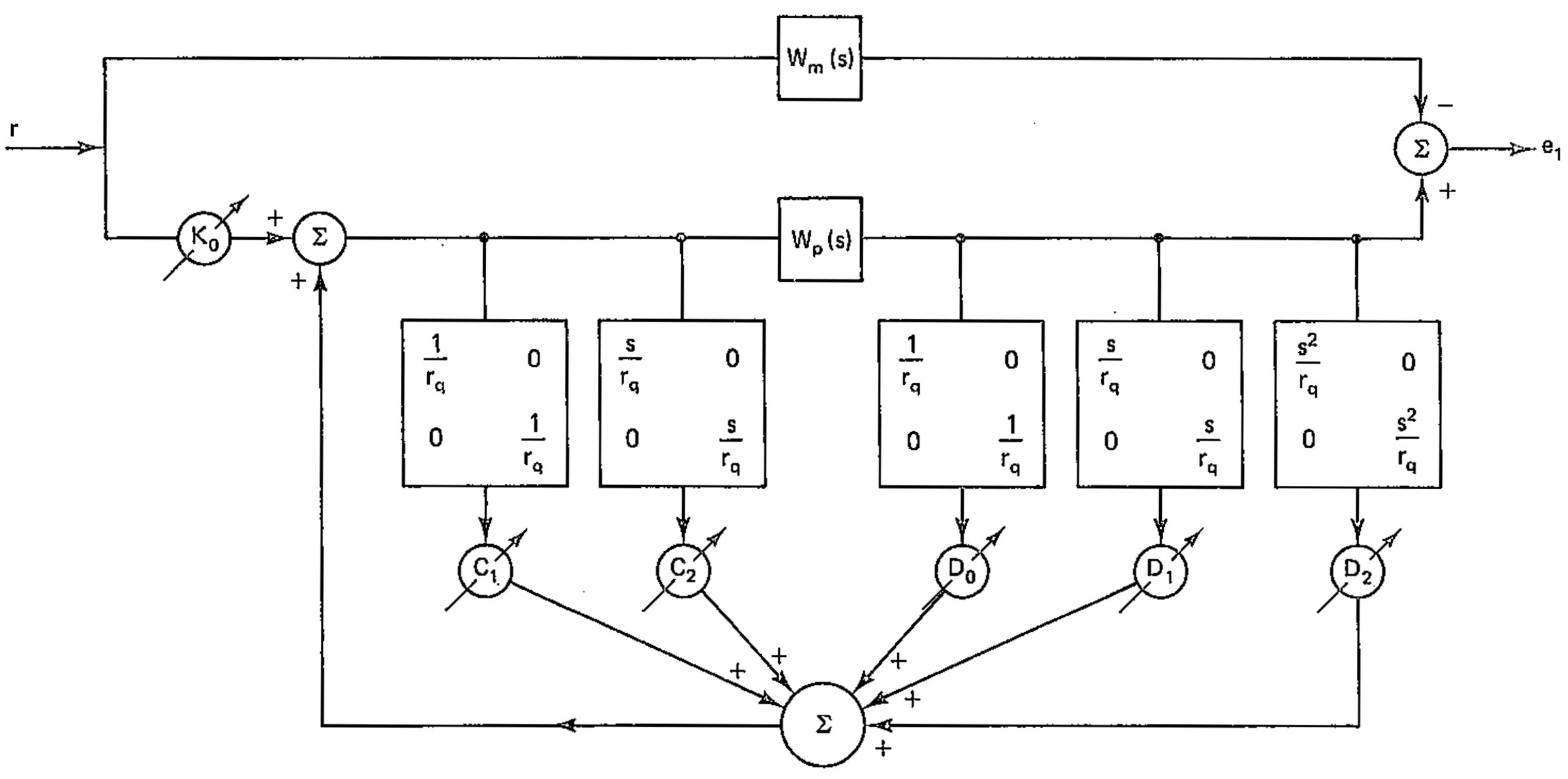
Each filter has a scalar denominator $r_{q}(s)$, and there are $m$ components to each filter, and a total of $2\nu-1$ filter, so the total number of integrations (i.e. the number of controller states) to generate the $\omega$ signals is $m(2\nu-1)$. There is a parameter matrix corresponding to each $\omega$ signal, giving $m^{2}(2\nu-1)$ parameters. See the following image from Reference ¹ p. 416. This block diagram provides a great way to see the structure of the control which otherwise might be a bit difficult given the construction and number of filters, and their corresponding adaptive elements.

With $\nu=$ this means there will be $2$ control input filters, and $3$ output filters. The denominator $r_{q}(s)$ can be selected as

\begin{equation}\label{eqn-adaptive-rqfilter} r_{q}(s)=s^{2}+s+1 \end{equation}

Control Input

Using the filtered control and outputs, the control input is given by

\begin{equation}\label{eqn-adaptive-control} u(t)=\Theta(t)\omega(t) \end{equation}

where

\begin{align*} \omega&= \begin{bmatrix} r & \omega_{1}^{\top} & \omega{2}^{\top} & \omega_{3}^{\top} & \omega{4}^{\top} & \omega{5}^{\top} \end{bmatrix}^{\top} \\ \Theta&= \begin{bmatrix} K_{0} & C_{1} & C_{2} & D_{0} & D_{1} & D_{2} \end{bmatrix} \end{align*}

Update Laws

With $H_{p}(s)$ strictly positive real, the update laws are given by

\begin{equation} \begin{aligned} \dot{K}_0&=-e_1r^{\top} & \qquad \dot{D}_0&=-e_1\omega_3^{\top} \\ \dot{C}_1&=-e_1\omega_1^{\top} & \qquad \dot{D}_1&=-e_1\omega_4^{\top} \\ \dot{C}_2&=-e_1\omega_2^{\top} & \qquad \dot{D}_2&=-e_1\omega_5^{\top} \end{aligned}\label{eqn-adaptive-updatelaws} \end{equation}

where $e_{1}=y_{p}-y_{m}$.

Controller Summary

The controller is complete with reference model in \eqref{eqn-adaptive-refmodel}, filter with denominator in \eqref{eqn-adaptive-rqfilter}, control law in \eqref{eqn-adaptive-control}, and update laws in \eqref{eqn-adaptive-updatelaws}.

Implementation in Python Control Systems Library

The simulation source is available at: https://github.com/dpwiese/control-examples/tree/master/classical-mimo. Defining the four linear components (plant, reference model, input and output filters) is straightforward with LinearIOSystem, using a state space representation in the case of the plant and transfer function in the case of the others.

 1
 2
 3
 4
 5
 6
 7
 8
 9
10
11
12
13
14
15
16
17
18
19
20
21
22
23
24
25
26
27
28
29
30
31
32
33
34
35
36
37
38
39

# Define plant
IO_PLANT = control.LinearIOSystem(
    control.StateSpace(A_P, B_P, C_P, D_P),
    inputs=2,
    outputs=2,
    states=5,
    name='plant'
)

# Define reference model
IO_REF_MODEL = control.LinearIOSystem(
    control.tf2ss(NUM_WM, DEN_WM),
    inputs=2,
    outputs=2,
    states=2,
    name='ref_model'
)

# Define input filters
# input: u
# outputs: omega_1, omega_2
IO_INPUT_FILTER = control.LinearIOSystem(
    control.tf2ss(NUM_IN, DEN_IN),
    inputs=2,
    outputs=4,
    states=4,
    name='input_filter'
)

# Define output filters
# input: y_p
# outputs: omega_3, omega_4, omega_5
IO_OUTPUT_FILTER = control.LinearIOSystem(
    control.tf2ss(NUM_OUT, DEN_OUT),
    inputs=2,
    outputs=6,
    states=4,
    name='output_filter'
)

The adaptive controller, being nonlinear, is defined using NonlinearIOSystem. The input to the adaptive controller is $\omega$, the state is the adaptive parameter $\Theta$, and the output is $u$. This allows the adaptive controller to be implemented as below.

 1
 2
 3
 4
 5
 6
 7
 8
 9
10
11
12
13
14
15
16
17
18
19
20
21
22
23
24
25
26
27
28
29
30
31
32
33
34
35
36
37
38
39
40
41
42
43
44
45
46
47
48

def adaptive_state(_t, x_state, u_input, _params):
    """Internal state of adpative controller"""

    # Algebraic Relationships: error: e_1 = y_p - y_m
    e_1_1 = u_input[12] - u_input[14]
    e_1_2 = u_input[13] - u_input[15]

    # Dynamics: update laws
    return [
        -e_1_1 * u_input[0],
        -e_1_2 * u_input[1],
        -e_1_1 * u_input[2],
        -e_1_2 * u_input[3],
        -e_1_1 * u_input[4],
        -e_1_2 * u_input[5],
        -e_1_1 * u_input[6],
        -e_1_2 * u_input[7],
        -e_1_1 * u_input[8],
        -e_1_2 * u_input[9],
        -e_1_1 * u_input[10],
        -e_1_2 * u_input[11]
        ]

def adaptive_output(_t, x_state, u_input, _params):
    """Algebraic output from adaptive controller"""

    # Define Theta and omega
    theta_1 = [x_state[0], x_state[2], x_state[4], x_state[6], x_state[8], x_state[10]]
    theta_2 = [x_state[1], x_state[3], x_state[5], x_state[7], x_state[9], x_state[11]]
    omega_1 = [u_input[0], u_input[2], u_input[4], u_input[6], u_input[8], u_input[10]]
    omega_2 = [u_input[1], u_input[3], u_input[5], u_input[7], u_input[9], u_input[11]]

    # Control law
    # u = Theta * omega
    return [
        sum([a*b for a, b in zip(theta_1, omega_1)]),
        sum([a*b for a, b in zip(theta_2, omega_2)])
        ]

IO_ADAPTIVE = control.NonlinearIOSystem(
    adaptive_state,
    adaptive_output,
    inputs=16,
    outputs=2,
    states=12,
    name='control',
    dt=0
)

Finally, the plant, reference model, input and output filters, and adaptive controller can be combined resulting in the following closed-loop system. Each pair of connections is of the form (<input>, <output>).

 1
 2
 3
 4
 5
 6
 7
 8
 9
10
11
12
13
14
15
16
17
18
19
20
21
22
23
24
25
26
27
28
29
30

# Define the closed-loop system
# x_cl = [plant[5], reference[2], input-filter[4], output_filter[4], controller[12]]
IO_CLOSED = control.InterconnectedSystem(
    (IO_PLANT, IO_REF_MODEL, IO_INPUT_FILTER, IO_OUTPUT_FILTER, IO_ADAPTIVE),
    connections=(
        ('plant.u[0]', 'control.y[0]'),
        ('plant.u[1]', 'control.y[1]'),
        ('input_filter.u[0]', 'control.y[0]'),
        ('input_filter.u[1]', 'control.y[1]'),
        ('output_filter.u[0]', 'plant.y[0]'),
        ('output_filter.u[1]', 'plant.y[1]'),
        ('control.u[2]', 'input_filter.y[0]'),
        ('control.u[3]', 'input_filter.y[1]'),
        ('control.u[4]', 'input_filter.y[2]'),
        ('control.u[5]', 'input_filter.y[3]'),
        ('control.u[6]', 'output_filter.y[0]'),
        ('control.u[7]', 'output_filter.y[1]'),
        ('control.u[8]', 'output_filter.y[2]'),
        ('control.u[9]', 'output_filter.y[3]'),
        ('control.u[10]', 'output_filter.y[4]'),
        ('control.u[11]', 'output_filter.y[5]'),
        ('control.u[12]', 'plant.y[0]'),
        ('control.u[13]', 'plant.y[1]'),
        ('control.u[14]', 'ref_model.y[0]'),
        ('control.u[15]', 'ref_model.y[1]')
    ),
    inplist=('ref_model.u[0]', 'ref_model.u[1]', 'control.u[0]', 'control.u[1]'),
    outlist=('plant.y[0]', 'plant.y[1]', 'ref_model.y[0]', 'ref_model.y[1]'),
    dt=0
)

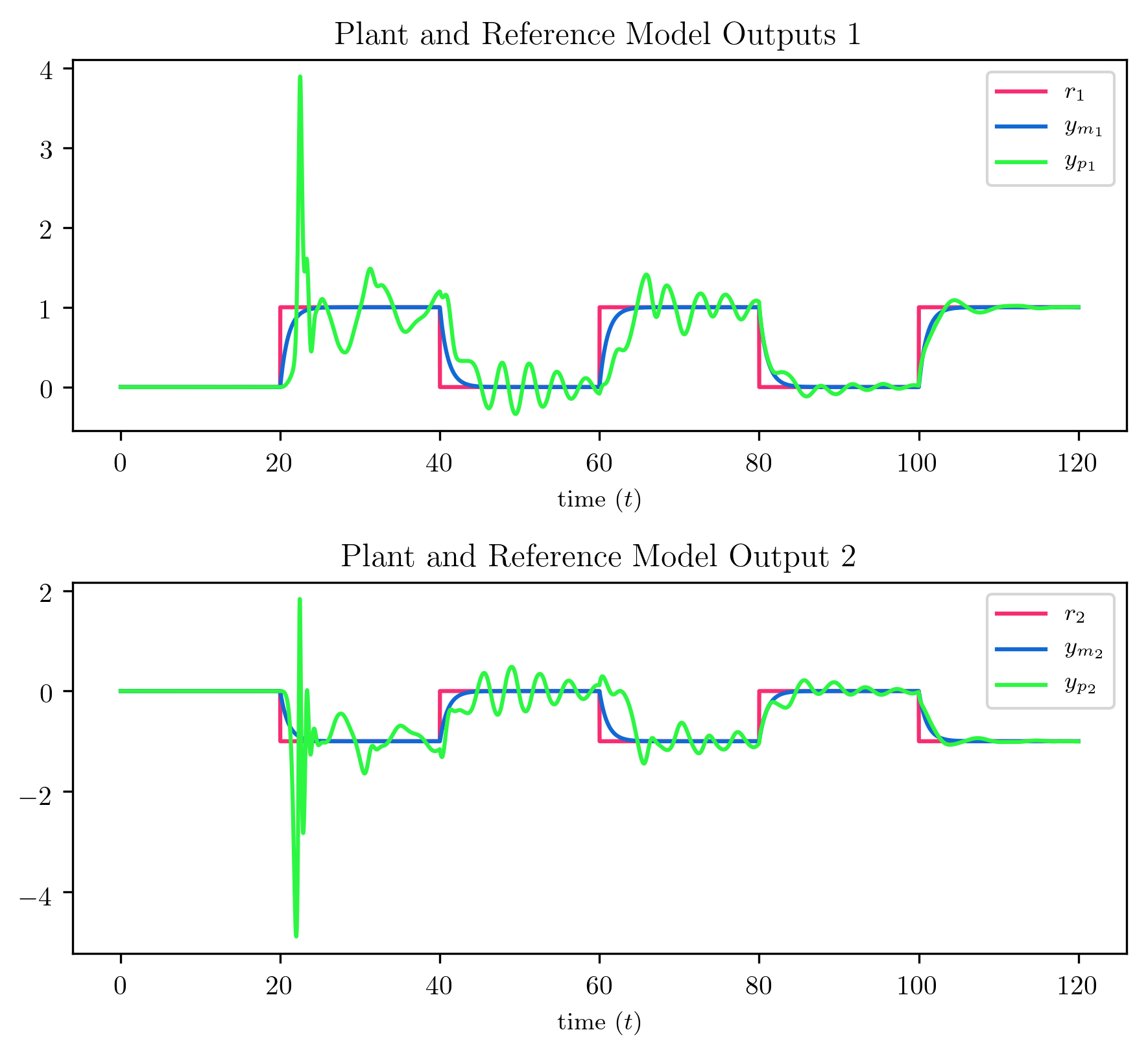
Simulation Result

The above closed loop system is simulated with input_output_response resulting in the following response.