Introduction

During graduate school I spent years studying, learning, and researching dynamic systems and adaptive learning and control theory. The majority of my work was theoretical - deriving new algorithms to learn about and control unique systems in new ways and prove that these algorithms would work. Theory was applied to determine how well such algorithms would work and understand the situations when they would fail. However, it was always interesting and useful to simulate the systems to actually see how they responded over time and gain additional insight into their performance. Almost every simulation was done in MATLAB/Simulink. Overall, I had a positive experience using these tools with expensive licenses provided to me for free during my tenure as a graduate student. Now several years out of school I thought it’d be nice to dig up some of the more interesting academic/classroom examples and make them available for others to use and learn from. However, I wanted to make sure these examples could be used for free, without requiring MATLAB/Simulink.

After a bit of searching around I found the Python Control Systems Library and was able to quickly implement a simple adaptive control example. I’ve been long meaning to write a post (or series of posts) introducing some interesting bits of system dynamics and control to the non-control engineer. This is not that post. I’m not going to attempt to introduce adaptive control or provide an accessible walkthrough of stability theory. This post will simply introduce a simple academic control problem, quickly work through the solution, and present a short code to simulate the system with the Python Control Systems Library. Even without a full understanding of the theory, it should be straightforward enough to see how the equations of interest are implemented in code and play with and modify the simulation. Hopefully this will serve at least as a starting point for others who may be interested in an open-source solution for simulating dynamic systems.

Speed Control of a DC Motor

Consider the following equation desribing the angular velocity $x$ of a DC motor, where the input $u$ is the motor torque. This model assumes motor torque is directly proportional to voltage and the fast electrical dynamics can be neglected.

\begin{equation} \label{eqn.adaptive.adaptivepi.gp} J\dot{x}+Bx=u \end{equation}

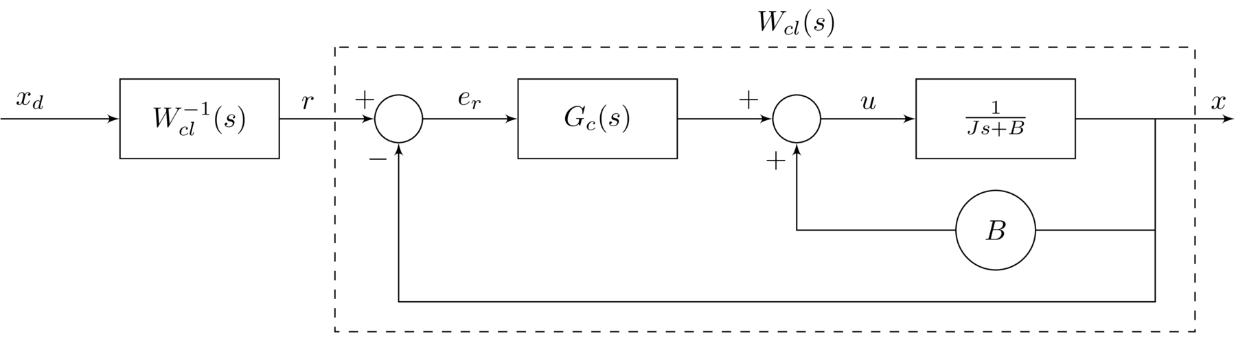
Note that because this is a motor, the rotational inertia $J>0$ and viscous damping $B>0$, giving the plant a stable pole at $−B/J$ and no zeros. This is a very simple system to consider for this control problem: first order, stable, and relative degree one. The control goal is: have $x\rightarrow x_{d}$ when the parameters $J$ and $B$ are unknown, where $x_{d}$ is the desired angular velocity. The controller will be connected with the plant as shown by the following block diagram

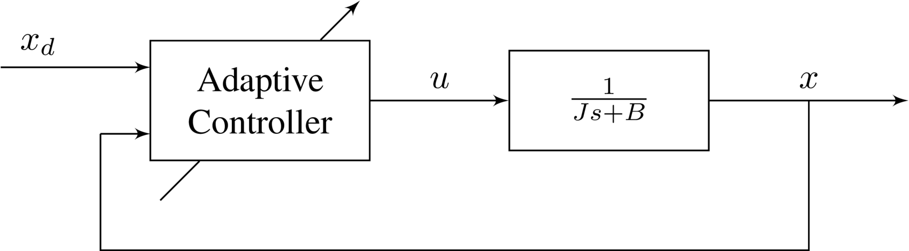
In the next section the control architecture is proposed.

Adaptive PI Control

The first step in the design of the adaptive PI controller is to first design the nominal PI controller: the PI controller that would designed if $J$ and $B$ were known. This is the algebraic solution. An adaptive version of this nominal controller is then created by replacing the parameter values within the controller with parameter estimates. This is the analytic solution. The procedure is an application of the certainty equivalence principle: develop a solution when the parameters are known, then replace the parameter values by their estimates. As these parameter estimates are learned adaptively in real time, stable update laws that govern their evolution must be determined.

Algebraic Solution

The following control architecture proposed, where in addition to the PI controller $G_{c}(s)$, and additional damping term is added. The need for this damping term may not be obvious, but completing the exercise below without this term will make its importance clear.

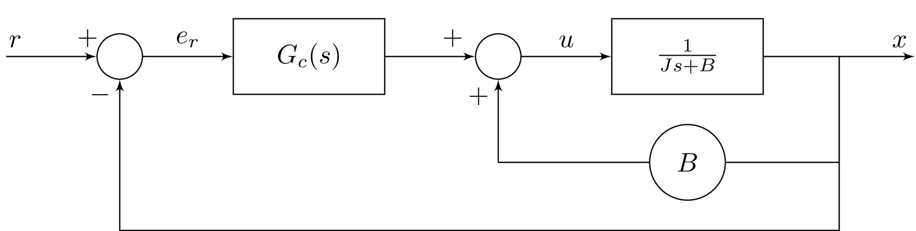
A standard PI controller is written in transfer function form as

\begin{equation*} G_{c}(s)=k_{p}+\frac{k_{i}}{s} \end{equation*}

where the control gains $k_{p}>0$ and $k_{i}>0$. This PI controller has a pole at the origin and a zero in the LHP at $-k_{i}/k_{p}$. The reference error $e_{r}$ is given by

\begin{equation*} e_{r}=r-x \end{equation*}

where $r$ is the reference input. A precompensator is proposed to generate $r$ from $x_{d}$. This is done by determining the closed-loop transfer function $W_{cl}(s)$ from $r$ to $x$ and defining the precompensator as the inverse. Thus, with the precompensator, the transfer function between $x_{d}$ and $x$ will be unity.

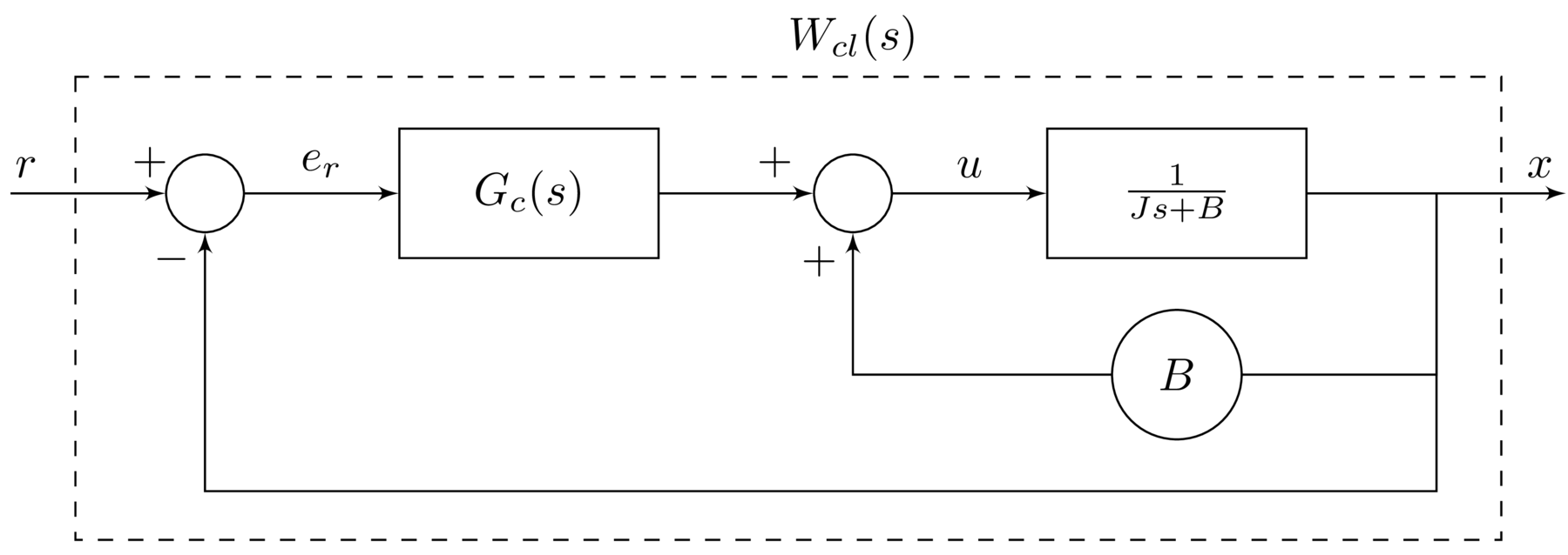
Evaluating $W_{cl}(s)$ gives

\begin{equation} \label{eqn.adaptive.adaptivepi.wcl} W_{cl}(s)=\frac{k_{p}s+k_{i}}{Js^{2}+k_{p}s+k_{i}} \end{equation}

From this the inverse can be found, and the reference input $r$ found in terms of the desired output $x_{d}$.

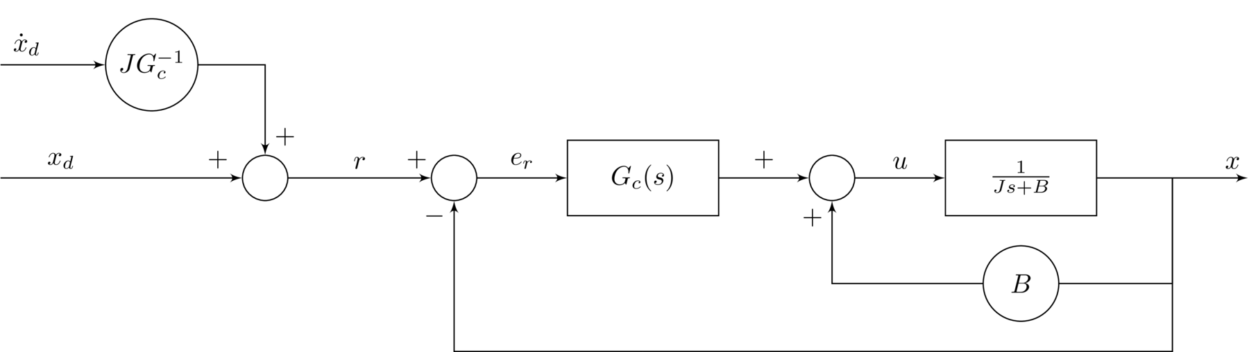
From $W_{cl}^{-1}(s)$, the reference input $r$ is given in terms of $x_{d}$ and $\dot{x}_{d}$ as

\begin{equation*} r=x_{d}+[JG_{c}^{-1}(s)]\dot{x}_{d} \end{equation*}

The block diagram can then be expressed as follows

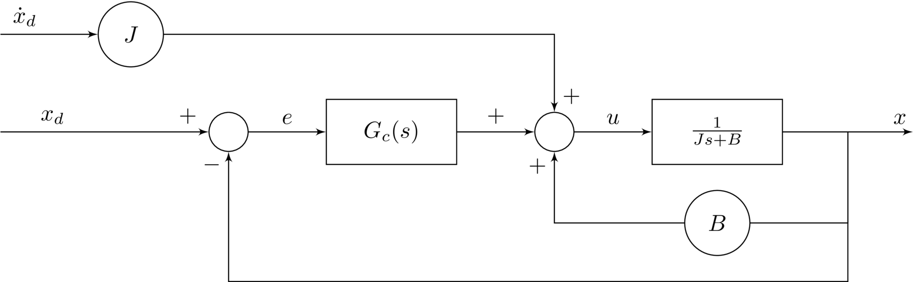
Equivalently, the input from $\dot{x}_{d}$ can be moved to better show how the control input $u$ is generated from the known signals.

The following parameterization is proposed

\begin{align*} k_{p}&=K+J\lambda{} \\ k_{i}&=K\lambda{} \end{align*}

where $K>0$ and $\lambda>0$. This reparameterization can be shown to make the damping ratio less dependent on uncertainties in $J$. This can be seen by comparing the closed loop transfer function in \eqref{eqn.adaptive.adaptivepi.wcl} with the reparameterized representation below.

\begin{equation*} W_{cl}(s)=\frac{(K+J\lambda)s+K\lambda}{Js^{2}+(K+J\lambda)s+K\lambda} \end{equation*}

Stability can be verified using the Routh-Hurwitz criterion: it will be stable if all of the coefficients of the characteristic polynomial have the same sign, which is of course the case given the non-negativity of the motor parameters and PI control gains.

\begin{equation*} J>0 \quad K>0 \quad \lambda>0 \end{equation*}

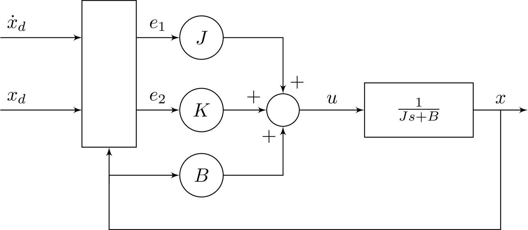
With the reparameterization the control input can be expressed

\begin{equation} \label{eqn.adaptive.adaptivepi.alglaw1} u=J(\dot{x}_{d}+\lambda e)+Bx+K\left(e+\lambda\int edt\right) \end{equation}

Defining the following errors

\begin{align} \label{eqn.adaptive.adaptivepi.e1} e_{1}&=\dot{x}_{d}+\lambda e \\ \label{eqn.adaptive.adaptivepi.e2} e_{2}&=e+\lambda\int edt \end{align}

allows the control law \eqref{eqn.adaptive.adaptivepi.alglaw1} to be written

\begin{equation} \label{eqn.adaptive.adaptivepi.alglaw2} u=Je_{1}+Bx+Ke_{2} \end{equation}

With the reparameterization and error definitions, the system can be expressed by the following block diagram.

This completes the algebraic solution. Given $J$ and $B$ known, the above controller perfectly inverts the internal dynamics consisting of the plant and PI controller, ensuring tracking of $x_{d}$ by $x$, as desired.

Analytic Solution

Now in the nominal control law in \eqref{eqn.adaptive.adaptivepi.alglaw2} that was proposed as the algebraic solution the unknown parameters $J$ and $B$ are replaced with their estimates, $\hat{J~}$ and $\hat{B~}$, respectively.

\begin{equation} \label{eqn.adaptive.adaptivepi.bettercontrollaw} u=\hat{J~}(t)e_{1}(t)+\hat{B~}(t)x(t)+Ke_{2}(t) \end{equation}

The block diagram is nearly identical as that in the algebraic solution, but using these parameter estimates instead.

Rearranging the plant dynamics from \eqref{eqn.adaptive.adaptivepi.gp} and substituting in the adaptive control law \eqref{eqn.adaptive.adaptivepi.bettercontrollaw} gives

\begin{equation*} \dot{x}=\frac{1}{J}\left(\tilde{B~}x+\hat{J~}e_{1}+Ke_{2}\right) \end{equation*}

where damping coefficient parameter error is

\begin{equation*} \tilde{B~}=\hat{B~}-B \end{equation*}

Differentiating the error $e$ gives

\begin{equation*} \dot{e}=\dot{x}_{d}-\frac{1}{J}\left(\tilde{B~}x+\hat{J~}e_{1}+Ke_{2}\right) \end{equation*}

Differentiating $e_{2}$ gives

\begin{equation} \label{eqn.adaptive.adaptivepi.e2dot} \dot{e}_{2}=-\frac{K}{J}e_2-\frac{1}{J}\left(\tilde{B~}x+\tilde{J~}e_1\right) \end{equation}

The following update laws are proposed

\begin{align} \label{eqn.adaptive.adaptivepi.update1} \dot{\tilde{J~}}&=\gamma_{1}e_{2}e_{1} \\ \label{eqn.adaptive.adaptivepi.update2} \dot{\tilde{B~}}&=\gamma_{2}e_{2}x \end{align}

With the error dynamics and update laws defined, stability must be proved.

Stability

Consider the following candidate Lyapunov function

\begin{equation*} V=\frac{1}{2}\left(Je_{2}^{2}+\frac{1}{\gamma_{1}}\tilde{J~}^{2}+\frac{1}{\gamma_{2}}\tilde{B~}^{2}\right) \end{equation*}

Differentiating and substituting the error dynamics in \eqref{eqn.adaptive.adaptivepi.e2dot} gives

\begin{equation*} \dot{V}=-Ke_{2}^{2}-\tilde{B~}xe_{2}-\tilde{J~}e_{1}e_{2}+\frac{1}{\gamma_{1}}\tilde{J~}\dot{\tilde{J~}}+\frac{1}{\gamma_{2}}\tilde{B~}\dot{\tilde{B~}} \end{equation*}

Using the update laws in \eqref{eqn.adaptive.adaptivepi.update1} and \eqref{eqn.adaptive.adaptivepi.update2} gives

\begin{equation} \label{eqn.adaptive.adaptivepi.vdot} \dot{V}=-Ke_{2}^{2} \end{equation}

Thus $\dot{V}\leq0$. With $e_{2}$, $\tilde{J~}$, $\tilde{B~}\in\mathcal{L}_{\infty} \Rightarrow \dot{e}_{2} \in\mathcal{L}_{\infty}$ by \eqref{eqn.adaptive.adaptivepi.e2dot}. And $e_{2}\in\mathcal{L}_{\infty} \Rightarrow e\in\mathcal{L}_{\infty}$ and $e\in\mathcal{L}_{\infty} \Rightarrow e_{1}\in\mathcal{L}_{\infty}$ by \eqref{eqn.adaptive.adaptivepi.e1} and \eqref{eqn.adaptive.adaptivepi.e2}. From \eqref{eqn.adaptive.adaptivepi.vdot} $e_{2}\in\mathcal{L}_{2}$ and using Barbalat's lemma this implies $\lim_{t\rightarrow\infty} e_{2}(t)=0 \Rightarrow \lim_{t\rightarrow\infty} e(t)=0$. Note that this result does not imply convergence of the parameter estimates to their true values.

System Summary

The closed-loop system can be described by the following equations.

\begin{align*} &\textbf{Plant:} &\hspace{0.5in} J\dot{x}+Bx&=u \\ &\textbf{Control:} & u&=\hat{J~}e_{1}+\hat{B~}x+Ke_{2} \\ &\textbf{Error:} & e&=x_{d}-x \\ & & e_{1}&=\dot{x}_{d}+\lambda{} e \\ & & e_{2}&=e+\lambda\int{} e(\tau)d\tau{} \\ &\textbf{Parameterization:} & k_{p}&=K+J\lambda{} \\ & & k_{i}&=K\lambda{} \\ &\textbf{Update laws:} & \dot{\hat{J~}}&=\gamma_{1}e_{2}e_{1} \\ & & \dot{\hat{B~}}&=\gamma_{2}e_{2}x \end{align*}

Simulation with the Python Control Systems Library

With the simple DC motor example above, the adaptive PI controller was proposed along with parameter estimate update laws, and stability proved. The system can now be implemented in a simulation to show how it actually responds. For this, the Python Control Systems Library is used. The implementation of the above system will be presented without great detail. The full code is available on Github: dpwiese/control-examples/adaptive-pi. Furthermore the documentation for the Python Control Systems Library is quite good.

The first step is defining the plant as a LinearIOSystem class, which, as the name suggests, represents a linear system. The parameters of the state-space representation of the plant described by \eqref{eqn.adaptive.adaptivepi.gp} are used. In creating the linear system the inputs, outputs, and state are described. The system is given a name to use when refering to its inputs and outputs.

1
2
3
4
5
6
7
8
9

SS_PLANT = control.StateSpace(-B/J, 1/J, 1, 0)

IO_DC_MOTOR = control.LinearIOSystem(
    SS_PLANT,
    inputs=('u'),
    outputs=('x'),
    states=('x'),
    name='plant'
)

Next, the controller is defined. As the controller is nonlinear, the NonlinearIOSystem class is used to describe it. The usage is very similar to that of linear systems, but requires defining an updfcn describing the state dynamics and an outfcn to return the output. These are adaptive_pi_state and adaptive_pi_output and are defined below.

1
2
3
4
5
6
7
8
9

IO_ADAPTIVE_PI = control.NonlinearIOSystem(
    adaptive_pi_state,
    adaptive_pi_output,
    inputs=3,
    outputs=('u', 'j_hat', 'b_hat'),
    states=3,
    name='control',
    dt=0
)

The state dynamics implements the integral error state in \eqref{eqn.adaptive.adaptivepi.e2} and the update laws in \eqref{eqn.adaptive.adaptivepi.update1} and \eqref{eqn.adaptive.adaptivepi.update2}. The output from this function are the equations which describe the evolution of the state via it’s derivatives.

 1
 2
 3
 4
 5
 6
 7
 8
 9
10
11
12
13
14
15
16
17
18
19
20
21
22

def adaptive_pi_state(_t, x_state, u_input, _params):
    """Internal state of adpative PI controller"""

    # Controller inputs
    x_d = u_input[0]
    x_d_dot = u_input[1]
    x = u_input[2]

    # Controller state
    e_i = x_state[2]

    # Algebraic relationships
    e = x_d - x
    e_1 = x_d_dot + LAMBDA * e
    e_2 = e + LAMBDA * e_i

    # Dynamics
    d_j_hat = GAMMA_1 * e_2 * e_1
    d_b_hat = GAMMA_2 * e_2 * x
    e_i_dot = e

    return [d_j_hat, d_b_hat, e_i_dot]

Next, the output function is defined, giving the output from the nonlinear adaptive controller. In this case, the controller output is just the control $u$ as given in \eqref{eqn.adaptive.adaptivepi.bettercontrollaw}, but the parameter estimates are returned as well for plotting.

 1
 2
 3
 4
 5
 6
 7
 8
 9
10
11
12
13
14
15
16
17
18
19
20
21
22

def adaptive_pi_output(_t, x_state, u_input, _params):
    """Algebraic output from adaptive PI controller"""

    # Controller inputs
    x_d = u_input[0]
    x_d_dot = u_input[1]
    x = u_input[2]

    # Controller state
    j_hat = x_state[0]
    b_hat = x_state[1]
    e_i = x_state[2]

    # Algebraic relationships
    e = x_d - x
    e_1 = x_d_dot + LAMBDA * e
    e_2 = e + LAMBDA * e_i

    # Control law
    u = j_hat * e_1 + b_hat * x + K * e_2

    return [u, j_hat, b_hat]

With the plant and controller defined, they only need to be connected and then the closed-loop system can be simulated. This is accomplished with the InterconnectedSystem class, that is explained well in the docs:

The InterconnectedSystem class is used to represent an input/output system that consists of an interconnection between a set of subystems. The outputs of each subsystem can be summed together to to provide inputs to other subsystems. The overall system inputs and outputs can be any subset of subsystem inputs and outputs.

In this example these interconnections are simple: the output of the controller control.u connects to the input of the plant plant.u, and the output of the plant plant.x connects to (one of) the controller inputs control.u[2]. The other two control inputs control.u[0] and control.u[1] are for the reference input and its derivative, $x_{d}$ and $\dot{x}_{d}$, respectively.

 1
 2
 3
 4
 5
 6
 7
 8
 9
10

IO_CLOSED = control.InterconnectedSystem(
    (IO_DC_MOTOR, IO_ADAPTIVE_PI),
    connections=(
        ('plant.u', 'control.u'),
        ('control.u[2]', 'plant.x')
    ),
    inplist=('control.u[0]', 'control.u[1]'),
    outlist=('plant.x', 'control.j_hat', 'control.b_hat'),
    dt=0
)

With the system configured, running the simulation is straightforward, only requiring the time steps T at which the input is defined, along with the input U at each time step, and the initial conditions X0.

1

T_OUT, Y_OUT = control.input_output_response(IO_CLOSED, T, U, X0)

Simulation Result

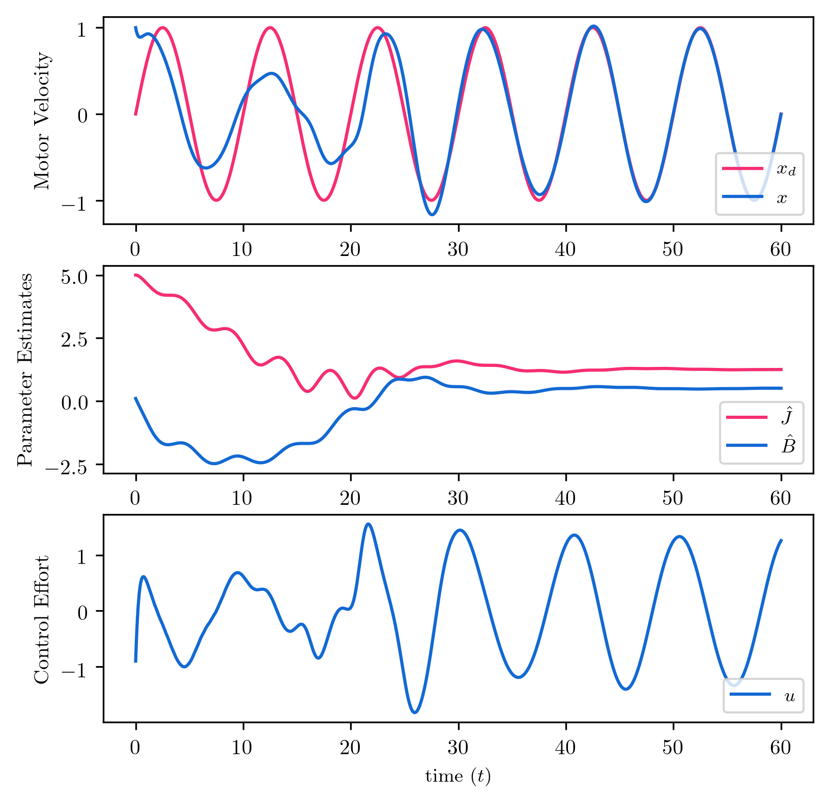
The results of the simulation are plotted using matplotlib and shown below. The initial motor velocity and parameter estimates are well of from their desired values. Tracking is poor and control effort somewhat erratic, although reasonable in magnitude, until about $t=30$ when the parameter estimates stability and tracking error approaches zero. To see how the system performs without adaptation, download the source code and try it out.