Introduction

This post presents some simple linear aircraft models and provides their implementation in Python for use with the Python Control Systems Library. Such models can be easily found across many references on aircraft flight mechanics, although these models typically vary slightly depending on the assumptions and simplifications made during their derivation. This post aims to provide some additional cohesion between these different models to better allow the variant best suited for use in control synthesis and simulation, and point to the various references which may be most useful.

Derivation from First Principles

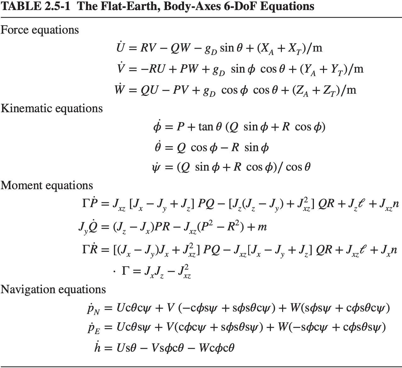
The derivation of the models begins with nothing more than Newton’s laws - the description of the motion of a body acted upon by forces and moments. In deriving these equations, some initial assumptions are commonly made for atmospheric flight vehicles - that the Earth is flat and nonrotating, and that the aircraft is a rigid body, thus neglecting the effects of rotating turbo machinery and sloshing fuel in the aircraft. Ref. ¹ presents these nonlinear equations in their matrix form in (eq. 1.7-18) and in scalar form as the twelve nonlinear differential equations in Table 2.5-1 shown below.

Ref. ² (Eq. 3.6-19 to 3.6-30) provides these twelve equations as well, albeit with slightly different notation.

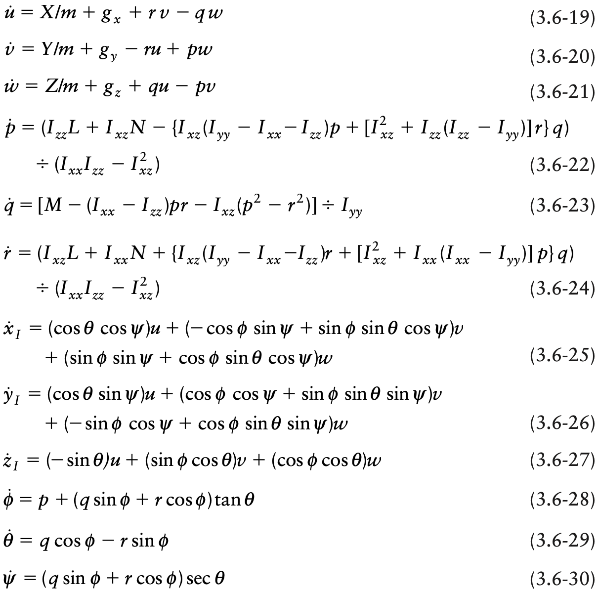
Ref. ³ Ch. 4 provide these equations as well, along with many of the references below. The state is the vehicle’s position and orientation along with its linear and angular velocity, each in three dimensions.

It is worth noting here that the axis system affixed to the vehicle is somewhat arbitrary. Its origin is at the center of gravity and the $x-z$ axes lie in the vehicles (assumed) plane of symmetry, but can be rotated about the $y$ axis. These general body-fixed axes are simply the datum that was chosen when designing the aircraft. So, while this selection is somewhat arbitrary, it is fixed to the aircraft and independent of flight condition.

Simplification of Nonlinear Equations

These equations, while some simplifications have already been made in deriving them, can be further simplified for many aerospace applications. The goal is often to linearize them about a desired flight condition and decouple the longitudinal and lateral-directional dynamics, resulting in the lowest order, linear system that appropriately models the aircraft. The validity of the linearization and decoupling can be verified to ensure such simplification is reasonable.

The next steps in simplification involves examining any quantities that can be neglected, and determining the functional dependence of the applied forces and moments (due to aerodynamic and propulsive forces).

The resulting linear equations will take the following matrix form

\begin{equation*} E\dot{x} = A^{\prime}x + B^{\prime}u \end{equation*}

where by left-multiplying both sides by $E^{-1}$ they can be written

\begin{equation*} \dot{x} = Ax + Bu \end{equation*}

This is the final state-space form of the equations as they are implemented for analysis and control synthesis. Selected outputs are given by:

\begin{equation*} y = Cx + Du \end{equation*}

Common Simplifications

The process of linearizing and simplifying the equations of motion is not presented in detail here. Rather, some of the common simplifications are stated, as the selected simplifications do vary somewhat between references. In the equations that follow, some of the “small” terms are retained in some instances and in others they are dropped. By listing at least some of the common simplifications here, the aim is to at least make obvious which terms should not be dropped.

Moments of Inertia

Assuming symmetry with respect to the $x-z$ plane results in only the $J_{xz}$ cross-product of inertia being nonzero ¹ (pg. 38). However, the $J_{xz}$ term is still generally very much smaller than $J_{xx}$, $J_{yy}$ and $J_{zz}$ and can often be neglected ⁴ (pg. 72).

Functional Dependence of Forces and Moments

Consider next the functional dependency of the forces and moments on the other variables, as this affects the presence of various partial derivative terms that result when linearizing. For example, assume the aircraft the force $X$ is a function of the following

\begin{equation*} X(u,w,q,\delta_{e},\delta_{\text{th}}) \end{equation*}

The dependence of $X$ on $u$, $w$, and $\delta_{\text{th}}$ are probably the most apparent ones, indicating essentially that the longitudinal force depends on airspeed, angle of attack, and thrust. That $X$ also depends sufficiently on the pitch rate $q$ and the elevator deflection angle are less obvious, but perhaps still appear reasonable. During linearization, partial derivative terms of $X$ will arise.

\begin{equation*} X_{i}=\frac{1}{m}\frac{\partial{}X}{\partial{}i} \end{equation*}

Given the assumed functional dependence of $X$, this would result in the following terms.

\begin{equation*} X_{u} \quad X_{w} \quad X_{q} \quad X_{\delta_{e}} \quad X_{\delta_{\text{th}}} \end{equation*}

By studying aircraft aerodynamic data it is found that many of the stability derivatives under most flight conditions can be neglected. Some such stability derivatives which are commonly neglected are the following, some of which are indicated in Ref. ⁵ (pg. 149) and Ref. ⁶ (pg. 33).

\begin{equation*} X_{\dot{u}} \quad X_{q} \quad X_{\dot{w}} \quad X_{\delta_{e}} \quad Z_{q} \quad Z_{\dot{u}} \quad Z_{\dot{w}} \quad M_{\dot{u}} \quad Z_{\dot{\delta_{e}}} \quad M_{\dot{\delta_{e}}} \end{equation*}

This neglecting of stability derivatives is another statement that there is not a strong functional dependence of the forces or moments on particular state variables or inputs and their derivatives.

Equilibrium Flight Condition

Finally, when linearizing the equations of motion, it is quite often the case that the equilibrium flight condition is steady, straight and level flight at cruise. This implies, among other things, that the pitch angle, angle of attack, and flight path angle are small, and the angle of sideslip, pitch rate, roll rate, and yaw rate are zero.

Longitudinal Dynamics

With some background presented on how, starting from Newton’s laws, simplified linear aircraft equations of motion can be derived, some simple models are presented.

General Body-Fixed Axes

The following, similar to that in Ref. ⁴ Eq. 4.65, is a standard 4-state longitudinal aircraft model, where the axes are the general body-fixed set described above. For the purposes of implementation, this model as suitable as-is. Values for a particular aircraft can be substituted into this form, and the inversion of $E$ can be performed numerically to achieve a model in standard state-space form.

\begin{equation} \label{eqn.exdotform.longitudinal} \begin{bmatrix} 1 & 0 & 0 & 0 \\ 0 & 1-Z_{\dot{w}} & 0 & 0 \\ 0 & -M_{\dot{w}} & 1 & 0 \\ 0 & 0 & 0 & 1 \end{bmatrix} \begin{bmatrix} \dot{u} \\ \dot{w} \\ \dot{q} \\ \dot{\theta} \end{bmatrix}= \begin{bmatrix} X_{u} & X_{w} & X_{q}-w_{\text{eq}} & -g\cos(\theta_{\text{eq}}) \\ Z_{u} & Z_{w} & Z_{q}+u_{\text{eq}} & -g\sin(\theta_{\text{eq}}) \\ M_{u} &M_{w} & M_{q} & 0 \\ 0 & 0 & 1 & 0 \end{bmatrix} \begin{bmatrix} u \\ w \\ q \\ \theta \end{bmatrix}+ \begin{bmatrix} X_{\delta_{\text{th}}} & X_{\delta_{e}} \\ Z_{\delta_{\text{th}}} & Z_{\delta_{e}} \\ M_{\delta_{\text{th}}} & M_{\delta_{e}} \\ 0 & 0 \end{bmatrix} \begin{bmatrix} \delta_{\text{th}} \\ \delta_{e} \end{bmatrix} \end{equation}

Analytical Simplification

For the purposes of comparing this model and its various terms to other models, it will be put in standard state-space form analytically. $E^{-1}$ is given by the following.

\begin{equation*} E^{-1}= \begin{bmatrix} 1 & 0 & 0 & 0 \\ 0 & \frac{1}{1-Z_{\dot{w}}} & 0 & 0 \\ 0 & \frac{M_{\dot{w}}}{1-Z_{\dot{w}}} & 1 & 0 \\ 0 & 0 & 0 & 1 \end{bmatrix} \end{equation*}

Performing the left multiplication by this inverse and assuming $Z_{\dot{w}}=0$ and $Z_{q}M_{\dot{w}}=0$ and $\sin(\theta_{\text{eq}})M_{\dot{w}}=0$ and $w_{\text{eq}}=0$ gives

\begin{equation*} \begin{bmatrix} \dot{u} \\ \dot{w} \\ \dot{q} \\ \dot{\theta} \end{bmatrix}= \begin{bmatrix} X_{u} & X_{w} & X_{q}-w_{\text{eq}} & -g\cos(\theta_{\text{eq}}) \\ Z_{u} & Z_{w} & Z_{q}+u_{\text{eq}} & -g\sin(\theta_{\text{eq}}) \\ M_{u}+M_{\dot{w}}Z_{u} & M_{w}+M_{\dot{w}}Z_{w} & M_{q}+M_{\dot{w}}u_{\text{eq}} & 0 \\ 0 & 0 & 1 & 0 \end{bmatrix} \begin{bmatrix} u \\ w \\ q \\ \theta \end{bmatrix}+ \begin{bmatrix} X_{\delta_{\text{th}}} & X_{\delta_{e}} \\ Z_{\delta_{\text{th}}} & Z_{\delta_{e}} \\ M_{\delta_{\text{th}}}+M_{\dot{w}}Z_{\delta_{\text{th}}} & M_{\delta_{e}}+M_{\dot{w}}Z_{\delta_{e}} \\ 0 & 0 \end{bmatrix} \begin{bmatrix} \delta_{\text{th}} \\ \delta_{e} \end{bmatrix} \end{equation*}

When additional assumptions are made, such as $\theta_{\text{eq}}=0$ and $w_{\text{eq}}=0$ and $X_{q}=0$ and $Z_{q}=0$ gives the following form, as in Ref. ⁵ Eq. 4.51.

\begin{equation} \label{eqn.ss.longitudinal.nelson} \begin{bmatrix} \dot{u} \\ \dot{w} \\ \dot{q} \\ \dot{\theta} \end{bmatrix}= \begin{bmatrix} X_{u} & X_{w} & 0 & -g \\ Z_{u} & Z_{w} & u_{\text{eq}} & 0 \\ M_{u}+M_{\dot{w}}Z_{u} & M_{w}+M_{\dot{w}}Z_{w} & M_{q}+M_{\dot{w}}u_{\text{eq}} & 0 \\ 0 & 0 & 1 & 0 \end{bmatrix} \begin{bmatrix} u \\ w \\ q \\ \theta \end{bmatrix}+ \begin{bmatrix} X_{\delta_{\text{th}}} & X_{\delta_{e}} \\ Z_{\delta_{\text{th}}} & Z_{\delta_{e}} \\ M_{\delta_{\text{th}}}+M_{\dot{w}}Z_{\delta_{\text{th}}} & M_{\delta_{e}}+M_{\dot{w}}Z_{\delta_{e}} \\ 0 & 0 \end{bmatrix} \begin{bmatrix} \delta_{\text{th}} \\ \delta_{e} \end{bmatrix} \end{equation}

Incorporation of Additional State Variables

Equations \eqref{eqn.exdotform.longitudinal} and \eqref{eqn.ss.longitudinal.nelson} are typical of linear longitudinal aircraft models. The four scalar state variables which describe the longitudinal dynamics of the aircraft are retained from the original twelve, providing a significantly simplified model. However, it may be the case that we wish to include altitude as a state in the model. Linearizing the altitude equation gives the following

\begin{equation*} \dot{h}=u_{\text{eq}}\theta-w \end{equation*}

Which can then be included in Equations \eqref{eqn.exdotform.longitudinal} as

\begin{equation*} \begin{bmatrix} 1 & 0 & 0 & 0 & 0 \\ 0 & 1-Z_{\dot{w}} & 0 & 0 & 0 \\ 0 & -M_{\dot{w}} & 1 & 0 & 0 \\ 0 & 0 & 0 & 1 & 0 \\ 0 & 0 & 0 & 0 & 1 \end{bmatrix} \begin{bmatrix} \dot{u} \\ \dot{w} \\ \dot{q} \\ \dot{\theta} \\ \dot{h} \end{bmatrix}= \begin{bmatrix} X_{u} & X_{w} & X_{q}-w_{\text{eq}} & -g\cos(\theta_{\text{eq}}) & 0 \\ Z_{u} & Z_{w} & Z_{q}+u_{\text{eq}} & -g\sin(\theta_{\text{eq}}) & 0 \\ M_{u} &M_{w} & M_{q} & 0 & 0 \\ 0 & 0 & 1 & 0 & 0 \\ 0 & -1 & 0 & u_{\text{eq}} & 0 \end{bmatrix} \begin{bmatrix} u \\ w \\ q \\ \theta \\ h \end{bmatrix}+ \begin{bmatrix} X_{\delta_{\text{th}}} & X_{\delta_{e}} \\ Z_{\delta_{\text{th}}} & Z_{\delta_{e}} \\ M_{\delta_{\text{th}}} & M_{\delta_{e}} \\ 0 & 0 \\ 0 & 0 \end{bmatrix} \begin{bmatrix} \delta_{\text{th}} \\ \delta_{e} \end{bmatrix} \end{equation*}

and similarly in \eqref{eqn.ss.longitudinal.nelson} as

\begin{equation*} \begin{bmatrix} \dot{u} \\ \dot{w} \\ \dot{q} \\ \dot{\theta} \\ \dot{h} \end{bmatrix}= \begin{bmatrix} X_{u} & X_{w} & 0 & -g & 0 \\ Z_{u} & Z_{w} & u_{\text{eq}} & 0 & 0 \\ M_{u}+M_{\dot{w}}Z_{u} & M_{w}+M_{\dot{w}}Z_{w} & M_{q}+M_{\dot{w}}u_{\text{eq}} & 0 & 0 \\ 0 & 0 & 1 & 0 & 0 \\ 0 & -1 & 0 & u_{\text{eq}} & 0 \end{bmatrix} \begin{bmatrix} u \\ w \\ q \\ \theta \\ h \end{bmatrix}+ \begin{bmatrix} X_{\delta_{\text{th}}} & X_{\delta_{e}} \\ Z_{\delta_{\text{th}}} & Z_{\delta_{e}} \\ M_{\delta_{\text{th}}}+M_{\dot{w}}Z_{\delta_{\text{th}}} & M_{\delta_{e}}+M_{\dot{w}}Z_{\delta_{e}} \\ 0 & 0 \\ 0 & 0 \end{bmatrix} \begin{bmatrix} \delta_{\text{th}} \\ \delta_{e} \end{bmatrix} \end{equation*}

Vertical acceleration is given in terms of general body-fixed axes as follows. See Ref. ⁶ (Eq. 2.94) and Ref. ⁴ (Eq. 4.5).

\begin{equation} \label{eqn.azcg} a_{z_{\text{cg}}} = \dot{w} - u_{\text{eq}}q \end{equation}

Substituting the expression for $\dot{w}$ this becomes an output equation in the form $y=Cx+Du$:

\begin{equation*} a_{z_{\text{cg}}} = Z_{u}u + Z_{w}w + Z_{\delta_{\text{th}}}\delta_{\text{th}} + Z_{\delta_{e}}\delta_{e} \end{equation*}

Short-Period Model

It is often the case that the four-state system in \eqref{eqn.ss.longitudinal.nelson} can be further separated into the short-period and phugoid modes. This is often presented in the literature without much justification, only that such separation is reasonable for many flight vehicles. In order to justify this separation for a particular flight vehicle, modal analysis is a helpful tool.

Modal Analysis

Modal analysis aims to determine which entries in a given eigenvector are small when the units of each state variable are not the same, so that the various modes may be decoupled. Ref. ⁷ Ch. 9 has a helpful section describing this process. Modal analysis allows \eqref{eqn.ss.longitudinal.nelson} to be decomposed into the short-period model below as in Ref. ⁵ (Eq. 4-71) or Ref. ⁸ (Eq. 11.56).

\begin{equation*} \begin{bmatrix} \dot{w} \\ \dot{q} \end{bmatrix}= \begin{bmatrix} Z_{w} & u_{\text{eq}} \\ M_{w}+M_{\dot{w}}Z_{w} & M_{q}+M_{\dot{w}}u_{\text{eq}} \end{bmatrix} \begin{bmatrix} w \\ q \end{bmatrix}+ \begin{bmatrix} Z_{\delta_{e}} \\ M_{\delta_{e}}+M_{\dot{w}}Z_{\delta_{e}} \end{bmatrix} \begin{bmatrix} \delta_{e} \end{bmatrix} \end{equation*}

As described above, different terms can be retained or neglected resulting in

\begin{equation} \label{eqn.ss.shortperiod.body} \begin{bmatrix} \dot{w} \\ \dot{q} \end{bmatrix}= \begin{bmatrix} Z_{w} & Z_{q}+u_{\text{eq}} \\ M_{w} & M_{q} \end{bmatrix} \begin{bmatrix} w \\ q \end{bmatrix}+ \begin{bmatrix} Z_{\delta_{e}} \\ M_{\delta_{e}} \end{bmatrix} \begin{bmatrix} \delta_{e} \end{bmatrix} \end{equation}

Stability Axes

Stability axes are another body-fixed axis system where the alignment of the axes is no longer the arbitrary aircraft designer’s datum. To affix the stability axes to the aircraft, an equilibrium flight condition is selected, and the axes are affixed such that the longitudinal stability axis points into the relative wind. After such a rotation, the $y$ and $z$ components of velocity in the general body-fixed axis system ($v$ and $w$, respectively) in the stability axis system become zero. Velocity is specified in terms of total velocity $V_{T}$ and the rotations about the lateral and vertical axis are the angle of attack and angle of sideslip.

Ref. ² Eq. 4.1-111a on pg. 492 has good rotation from the general body-fixed reference frame to stability axis system and gives the small angle approximation in Eq. 4.1-111b. Consider \eqref{eqn.ss.shortperiod.body} below.

\begin{equation*} \begin{split} \dot{w} &= Z_{w}w + (Z_{q}+u_{\text{eq}})q + Z_{\delta_{e}}\delta_{e} \\ \dot{q} &= M_{w}w + M_{q}q + M_{\delta_{e}}\delta_{e} \end{split} \end{equation*}

Using the following substitutions

\begin{equation} \label{eqn.stabilitysubs} u_{\text{eq}} = V_{\text{eq}} \qquad w = V_{\text{eq}}\alpha \qquad \dot{w} = V_{\text{eq}}\dot{\alpha} \qquad u = V_{T} \end{equation}

Gives

\begin{equation*} \begin{split} \dot{\alpha} &= \frac{Z_{\alpha}}{V_{\text{eq}}}\alpha + (1+\frac{Z_{q}}{V_{\text{eq}}})q + \frac{Z_{\delta_{e}}}{V_{\text{eq}}}\delta_{e} \\ \dot{q} &= M_{\alpha}\alpha + M_{q}q + M_{\delta_{e}}\delta_{e} \end{split} \end{equation*}

where

\begin{equation*} Z_{\alpha} = Z_{w}V_{\text{eq}} \qquad M_{\alpha} = M_{w}V_{\text{eq}} \end{equation*}

Putting these into state-space form we get Ref. ⁹ Eq. 1.8

\begin{equation*} \begin{bmatrix} \dot{\alpha} \\ \dot{q} \end{bmatrix}= \begin{bmatrix} \frac{Z_{\alpha}}{V_{\text{eq}}} & 1+\frac{Z_{q}}{V_{\text{eq}}} \\ M_{\alpha} & M_{q} \end{bmatrix} \begin{bmatrix} \alpha \\ q \end{bmatrix}+ \begin{bmatrix} \frac{Z_{\delta_{e}}}{V_{\text{eq}}} \\ M_{\delta_{e}} \end{bmatrix} \delta_{e} \end{equation*}

Ref. ⁵ Eq. 4.75 presents the short-period model as well, although neglecting and retaining a couple terms different than Ref. ⁹.

Incorporation of Additional State Variables

The transformation of any of the higher order models (those including velocity, pitch angle, and altitude, for example) can also be converted to the stability axis system as in Ref. ⁹ Eq. 1.7 below. Note the equilibrium flight path angle, $\gamma_{\text{eq}}$, is calculated using $\gamma = \theta - \alpha$.

\begin{equation*} \begin{bmatrix} \dot{V_{T}} \\ \dot{\alpha} \\ \dot{q} \\ \dot{\theta} \end{bmatrix}= \begin{bmatrix} X_{V} & X_{\alpha} & 0 & -g\cos(\gamma_{\text{eq}}) \\ \frac{Z_{V}}{V_{\text{eq}}} & \frac{Z_{\alpha}}{V_{\text{eq}}} & 1+\frac{Z_{q}}{V_{\text{eq}}} & \frac{-g\sin(\gamma_{\text{eq}})}{V_{\text{eq}}} \\ M_{V} & M_{\alpha}+\frac{M_{\dot{\alpha}}Z_{\alpha}}{V_{\text{eq}}} & M_{q}+M_{\dot{\alpha}} & 0 \\ 0 & 0 & 1 & 0 \\ \end{bmatrix} \begin{bmatrix} V_{T} \\ \alpha \\ q \\ \theta \end{bmatrix}+ \begin{bmatrix} X_{\delta_{\text{th}}}\cos(\alpha_{\text{eq}}) & X_{\delta_{e}} \\ -X_{\delta_{\text{th}}}\sin(\alpha_{\text{eq}}) & \frac{Z_{\delta_{e}}}{V_{\text{eq}}} \\ M_{\delta_{\text{th}}} & M_{\delta_{e}} \\ 0 & 0 \end{bmatrix} \begin{bmatrix} \delta_{\text{th}} \\ \delta_{e} \end{bmatrix} \end{equation*}

This can be extended with altitude as in Ref. ⁹ Eq. 1.10

\begin{equation*} \dot{h}=V_{\text{eq}}(\theta-\alpha) \end{equation*}

Giving

\begin{equation*} \begin{bmatrix} \dot{V_{T}} \\ \dot{\alpha} \\ \dot{q} \\ \dot{\theta} \\ \dot{h} \end{bmatrix}= \begin{bmatrix} X_{V} & X_{\alpha} & 0 & -g\cos(\gamma_{\text{eq}}) & 0 \\ \frac{Z_{V}}{V_{\text{eq}}} & \frac{Z_{\alpha}}{V_{\text{eq}}} & 1+\frac{Z_{q}}{V_{\text{eq}}} & \frac{-g\sin(\gamma_{\text{eq}})}{V_{\text{eq}}} & 0 \\ M_{V} & M_{\alpha}+\frac{M_{\dot{\alpha}}Z_{\alpha}}{V_{\text{eq}}} & M_{q}+M_{\dot{\alpha}} & 0 & 0 \\ 0 & 0 & 1 & 0 & 0 \\ 0 & -V_{\text{eq}} & 0 & V_{\text{eq}} & 0 \end{bmatrix} \begin{bmatrix} V_{T} \\ \alpha \\ q \\ \theta \\ h \end{bmatrix}+ \begin{bmatrix} X_{\delta_{\text{th}}}\cos(\alpha_{\text{eq}}) & X_{\delta_{e}} \\ -X_{\delta_{\text{th}}}\sin(\alpha_{\text{eq}}) & \frac{Z_{\delta_{e}}}{V_{\text{eq}}} \\ M_{\delta_{\text{th}}} & M_{\delta_{e}} \\ 0 & 0 \\ 0 & 0 \end{bmatrix} \begin{bmatrix} \delta_{\text{th}} \\ \delta_{e} \end{bmatrix} \end{equation*}

Vertical acceleration in stability axes can be obtained using \eqref{eqn.azcg} with the substitutions in \eqref{eqn.stabilitysubs} giving

\begin{equation*} a_{z_{\text{cg}}} = Z_{V}V_{T} + Z_{\alpha}\alpha + Z_{q}q - g\sin(\gamma_{\text{eq}})\theta - V_{\text{eq}}X_{\delta_{\text{th}}}\sin(\alpha_{\text{eq}})\delta_{\text{th}} + Z_{\delta_{e}}\delta_{e} \end{equation*}

Lateral-Directional Dynamics

In the same way that the full, twelve state, nonlinear equations of motion were linearized and the longitudinal variables separated out, the same can be done for the lateral-directional equations. This separation can be confirmed for most flight vehicles using modal analysis.

General Body-Fixed Axes

See for example the following model as in Ref. ⁴ Example 4.4 (pg. 90).

\begin{equation*} \begin{bmatrix} 1 & 0 & 0 & 0 \\ 0 & 1 & -\frac{J_{xz}}{J_{xx}} & 0 \\ 0 & -\frac{J_{xz}}{J_{zz}} & 1 & 0 \\ 0 & 0 & 0 & 1 \end{bmatrix} \begin{bmatrix} \dot{v} \\ \dot{p} \\ \dot{r} \\ \dot{\phi} \end{bmatrix}= \begin{bmatrix} Y_{v} & Y_{p} & Y_{r}-u_{\text{eq}} & -g\cos(\theta_{\text{eq}}) \\ L_{v} & L_{p} & L_{r} & 0 \\ N_{v} & N_{p} & N_{r} & 0 \\ 0 & 1 & 0 & 0 \end{bmatrix} \begin{bmatrix} v \\ p \\ r \\ \phi \end{bmatrix}+ \begin{bmatrix} Y_{\delta_{a}} & Y_{\delta_{r}} \\ L_{\delta_{a}} & L_{\delta_{r}} \\ N_{\delta_{a}} & N_{\delta_{r}} \\ 0 & 0 \end{bmatrix} \begin{bmatrix} \delta_{a} \\ \delta_{r} \end{bmatrix} \end{equation*}

When this equation is left-multiplied by $E^{-1}$ a form such as that in Ref. ⁵ (Eq. 5.33) is obtained. Neglecting $J_{xz}$ makes $E$ and its inverse the identity matrix.

Stability Axes Systems

In converting between the general body-fixed and stability axes, the axes are rotated about the lateral $y$ axis of the aircraft. In the longitudinal case, this doesn’t result in any transformation between the pitch rate depending on the axes used. In the lateral-directional case, the angular rates must be expressed differently when using stability axes. Ref. ⁴ (Eq. 2.12) gives the direction cosine matrix that can be used to accomplish such transformation resulting in Ref. ⁷ (Eq. 7.7). However, assuming small angles results in the approximation of these angular rates being equivalent in both axes systems.

The result is a state-space representation such as Ref. ¹⁰ (Eq. 2.14) or ⁵ (Eq. 5.35) below.

\begin{equation*} \begin{bmatrix} \dot{\beta} \\ \dot{p} \\ \dot{r} \\ \dot{\phi} \\ \dot{\psi} \end{bmatrix}= \begin{bmatrix} \frac{Y_{\beta}}{V_{\text{eq}}} & \frac{Y_{p}}{V_{\text{eq}}} & \frac{Y_{r}}{V_{\text{eq}}}-1 & \frac{g\cos(\theta_{\text{eq}})}{V_{\text{eq}}} & 0 \\ L_{\beta} & L_{p} & L_{r} & 0 & 0\\ N_{\beta} & N_{p} & N_{r} & 0 & 0 \\ 0 & 1 & 0 & 0 & 0 \\ 0 & 0 & 1 & 0 & 0 \end{bmatrix} \begin{bmatrix} \beta \\ p \\ r \\ \phi \\ \psi \end{bmatrix}+ \begin{bmatrix} \frac{Y_{\delta_{a}}}{V_{\text{eq}}} & \frac{Y_{\delta_{r}}}{V_{\text{eq}}} \\ L_{\delta_{a}} & L_{\delta_{r}} \\ N_{\delta_{a}} & N_{\delta_{r}} \\ 0 & 0 \\ 0 & 0 \end{bmatrix} \begin{bmatrix} \delta_{a} \\ \delta_{r} \end{bmatrix} \end{equation*}

where

\begin{equation*} Y_{\beta} = Y_{v}V_{\text{eq}} \qquad L_{\beta} = L_{v}V_{\text{eq}} \qquad N_{\beta} = N_{v}V_{\text{eq}} \end{equation*}

Implementation in Python

The implementation of the above models for use in the Python Control Systems Library is straightforward. The equilibrium flight condition, mass properties, and stability and control derivatives for the vehicle must be defined. These are usually available in the references below for a variety of different aircraft. Then, the for matrices $A$, $B$, $C$, and $D$ of the desired model must be populated with these values. See dpwiese/control-examples/aircraft-dynamics on Github.